#include "fs_common.h"
#include "ldz_gradpe.hpp"
#include <limits>

Include dependency graph for ldz_gradpe.cpp:

Functions
void	calculateGradPeTerm (fsgrids::egradpespan egradpes, fsgrids::constmomentsspan moments, fsgrids::constdmomentsspan dmoments, fsgrids::consttechnicalspan technical, const fsgrid::FsStencil &stencil, const auto &gridSpacing, SysBoundary &sysBoundaries)
void	calculateGradPeTermSimple (fsgrids::egradpespan egradpe, fsgrids::egradpespan egradpedt2, fsgrids::momentsspan moments, fsgrids::momentsspan momentsdt2, fsgrids::dmomentsspan dmoments, fsgrids::dmomentsspan dmomentsdt2, fsgrids::technicalspan technical, FieldSolverGrid &fsgrid, SysBoundary &sysBoundaries, cint &RKCase)

Function Documentation

◆ calculateGradPeTerm()

void calculateGradPeTerm	(	fsgrids::egradpespan	egradpes,
		fsgrids::constmomentsspan	moments,
		fsgrids::constdmomentsspan	dmoments,
		fsgrids::consttechnicalspan	technical,
		const fsgrid::FsStencil &	stencil,
		const auto &	gridSpacing,
		SysBoundary &	sysBoundaries )

Vlasiator considers electrons an inertia-free charge-neutralizing fluid. To model the effects of electron pressure on plasma dynamics (such as the cross-shock potential, an electric field induced by electron pressure changes), we consider the electron pressure gradient term in the generalized Ohm's law:

nabla dot P_e /(n_e e)

To model this, we can assume some equation of state for electrons. We now assume that the electron fluid has an isotropic pressure tensor (so pressure is a scalar), and that it is governed by a polytropic process, where P * V^k is constant. Here P is the pressure, V is the volume of an unit of fluid, and k is a polytropic index describing the process.

Using this equation, for any position in the simulation, the electron temperature can be evaluated based on the local electron number density (assumed to be equal to the ion charge density fsgrids::moments::RHOQ divided by the elementary charge) and some normalization or anchoring values.

The polytropic index can be, e.g.: k = 0 : Isobaric process (pressure is constant) k = 1 : Isothermal process (temperature is constant) k = gamma : Adiabatic process (no energy transfer)

Here gamma is the ratio of specific heats, that is the heat capacity at constant pressure (C_P) divided by the heat capacity at constant volume (C_V). For an ideal monoatomic gas, gamma = 5/3.

Now because P * V^k is constant, we can evaluate that constant for the whole simulation based on the values at some hypothetical anchor point, with values usually declared based on the upstream inflow conditions. These values are only used for normalizing the relationship between electron density and electron temperature for the given polytropic relation. These anchor point values are provided by the user as config parameters - the anchor point is not an actual physical point in the simulation, but just imagined for normalization purposes..

Example in a cfg-script: [fieldsolver] ohmGradPeTerm = 1 # active electronPTindex = 1.666667 # adiabatic, 3/2 electronDensity = 1.0e6 # anchor point (here: inflow solar wind) electron density value electronTemperature = 0.125e6 # electron temperature associated with the anchor point density value. Here

the value is set to 1/4 of the solar wind proton temperature.

The user may, for example, use inflow solar wind electron values as the anchor point values. A good rule of thumb is that electron number density times elementary charge should match the ion charge density in the solar wind. A zeroth-order approximation is to set electron temperature to equal that of solar wind ions, but alternatively an observation-based factor (e.g. 0.25) may be applied to decrease electron temperatures at the anchor point.

In derivatives.cpp we first calculate the electron pressure at this anchor point: Real Pe_anchor = Parameters::electronTemperature * Parameters::electronDensity * physicalconstants::K_B; And then calculate the constant used further on: Real Pe_const = Pe_anchor * pow(Parameters::electronDensity, -Parameters::electronPTindex);

Remembering that P * V^k = P * (n_e)^-k is constant, we can calculate that constant from the anchor point values, and use that for solving the electron pressure at any given position as P(r) = Pe_const * (n_e(r))^k

Thus, the gradient of electron pressure is calculated in derivatives.cpp using a standard slope limiter, for each Cartesian direction.

Note: The value stored in e.g. dMomentsGrid.get(i,j,k)->at(fsgrids::dmoments::drhoqdx) is a difference, not a derivative. Thus, in the next step, evaluating the electron pressure gradient term in the general Ohm's law as E_gradPe(x,y,z) = - dPe/d(x,y,z) / (n_e * e * Delta(x,y,z)) requires adding EGradPeGrid.DX/DY/DZ in the denominator.

Similar to the Hall term, we use the Parameters::hallMinimumRhoq value as a lower bound for electron number density in order to prevent runaway electric field terms at depletion zones. Calculate the electron pressure gradient term on all given cells.

Parameters

egradpes	fsgrid of Hall term electric fields
moments	fsgrid of moments
dmoments	fsgrid of moments derivatives
technical	fsgrid with technical parameters
stencil	fsgrid stencil of current cell
gridSpacing	fsgrid cell size in x,y,z
sysBoundaries	System boundary condition functions.

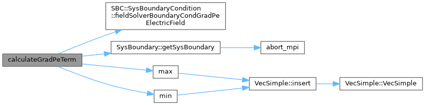
Definition at line 107 of file ldz_gradpe.cpp.

Here is the call graph for this function:

Here is the caller graph for this function:

◆ calculateGradPeTermSimple()

void calculateGradPeTermSimple	(	fsgrids::egradpespan	egradpe,
		fsgrids::egradpespan	egradpedt2,
		fsgrids::momentsspan	moments,
		fsgrids::momentsspan	momentsdt2,
		fsgrids::dmomentsspan	dmoments,
		fsgrids::dmomentsspan	dmomentsdt2,
		fsgrids::technicalspan	technical,
		FieldSolverGrid &	fsgrid,
		SysBoundary &	sysBoundaries,
		cint &	RKCase )

Definition at line 157 of file ldz_gradpe.cpp.